CoachellaR - A Cluster Analysis

Scraping the Coachella Website for Artists

From the lineup page, I found the lineup-listing element and pulled it down as a character, then extracted just the individual JSON entries with regex into a character vector.

library(tidyverse)
library(rvest)
library(stringr)

### grab coachella artist info
baseurl <- 'https://www.coachella.com/lineup/'
base <- read_html(baseurl)

node <- base %>%
    xml_node('#main') %>%
    xml_node('lineup-listing') %>%
    as.character

coachella <- regmatches(node, gregexpr("(?:\\{).*?(?<:\\})", node, perl:T))[[1]]

str(coachella)

chr [1:397] "{\"id\":\"1982\",\"name\":\"Alison Swing\",\"biography\":null,\"image_url\"..."

I noticed that each artist had one long entry containing both general info and data on their first weekend. Most artists, who play both weekends, had a second, smaller entry with just info on their second weekend. Since I was just interested in the raw artist data, I looped through all entries and kept only the long ones (as of this writing, those with over 400 characters sufficed), using jsonlite to convert to a data.frame.

library(jsonlite)

coachella_df <- map_df(seq(1, length(coachella)), function(x) {
    if (nchar(coachella[x]) <: 400) {
        return(data.frame()) ## skip elements with small amounts of text (they're event info for weekend 2)
    }
    json <- paste0('[', coachella[x], '}}]') ## add brackets to complete json format
    fromJSON(json)
})

str(select(coachella_df, -events))

'data.frame':   229 obs. of  18 variables:
 $ id                : chr  "1982" "1983" "2149" "2214" ...
 $ name              : chr  "Alison Swing" "Allah-Las" "Amtrac" "Andre Power" ...
 $ biography         : chr  NA NA NA "" ...
 $ image_url         : chr  "https://s3.amazonaws.com/gv-account-assets/artist-images/" ...
 $ website_url       : chr  "https://soundcloud.com/alisonswing" "http://allah-las.com/" ...
 $ facebook_url      : chr  "https://www.facebook.com/alisonswing" "https://www.facebook.com/" ...
 $ twitter_url       : chr  "https://twitter.com/alisonswing" "https://twitter.com/AllahLas" ...
 $ youtube_url       : chr  "" "https://www.youtube.com/channel/UCRg0dGQ51ZX7b3SF-6HkMDA" ...
 $ instagram_url     : chr  "https://www.instagram.com/alisonswing/" "https://www.instagram.com/"
 $ deleted           : chr  "0" "0" "0" "0" ...
 $ spotify_track_uri : logi  NA NA NA NA NA NA ...
 $ spotify_url       : chr  NA NA NA NA ...
 $ festival_year     : chr  "2017" "2017" "2017" "2017" ...
 $ livestream_channel: chr  NA NA NA NA ...
 $ livestream_start  : chr  NA NA NA NA ...
 $ livestream_end    : chr  NA NA NA NA ...
 $ tumblr_url        : logi  NA NA NA NA NA NA ...
 $ apple_url         : chr  "" "https://itunes.apple.com/us/artist/allah-las/id4267682" ...

 length(coachella_df$events)
 [1] 229

 str(coachella_df$events[1])
 List of 1
 $ :'data.frame':   1 obs. of  15 variables:
  ..$ id                : chr "2415"
  ..$ artist_id         : chr "1982"
  ..$ event_location_id : chr "16"
  ..$ weekend           : chr "1"
  ..$ event_date        : chr "2017-04-14"
  ..$ start_time        : chr "14:00:00"
  ..$ end_time          : chr "15:30:00"
  ..$ deleted           : chr "0"
  ..$ festival_year     : chr "2017"
  ..$ location          : chr "Yuma"
  ..$ date_time         : chr "Friday, April 14, 2017"
  ..$ start_time_app    : chr "2017-04-14 14:00:00"
  ..$ end_time_app      : chr "2017-04-14 15:30:00"
  ..$ start_time_display: chr "02:00 PM"
  ..$ end_time_display  : chr "03:30 PM"

The first thing that jumped out was how rich the dataset was. The tech team at Coachella put a ton of information in here, including the channels to watch the livestreams on.

Before getting Spotify audio features I had to clean up the artist names a bit, such as accounting for dual acts like “Porter Robinson & Madeon.” In these cases, I separated the two artists and pulled their song data separately. Then I averaged them together for the final analysis.

artists <- select(coachella_df, name, id) %>% mutate(name : str_trim(name))
artists$name[artists$name :: 'R&amp;ouml;yksopp'] <- 'Röyksopp'
artists$name[artists$name :: 'R&amp;oacute;is&amp;iacute;n Murphy'] <- 'Róisín Murphy'
artists$name[artists$name :: 'Richie Hawtin Close'] <- 'Richie Hawtin'
artists$name[artists$name :: 'Josh Billings and Nonfiction'] <- 'Josh Billings'
artists$name[artists$name :: 'Porter Robinson &amp; Madeon'] <- 'Porter Robinson'
artists$name[artists$name :: 'Gaslamp Killer'] <- 'The Gaslamp Killer'
artists$name[artists$name :: 'HAANA'] <- 'HÄANA'
artists$name[artists$name :: 'Toots and the Maytals'] <- 'Toots & The Maytals'
artists$name[grepl('&amp;', artists$name)] <- gsub('&amp;', '&', artists$name[grepl('&amp;', artists$name)])

artists <- rbind(artists, tibble(name : c('Nonfiction', 'Madeon'), id : c(NA, NA)))

head(artists)

          name   id
1 Alison Swing 1982
2    Allah-Las 1983
3       Amtrac 2149
4  Andre Power 2214
5   Anna Lunoe 1984
6      Arkells 1985

Spotify Web API

To classify each artist, I pulled the audio features for their top 10 most popular songs on Spotify in the U.S. as of April 14th, 2017. This took three steps for each artist: 1. Find the Spotify Artist URI 2. Get their top 10 most popular U.S. tracks 3. Pull the audio features for each track

For Step 1, I created a function to hit Spotify’s search endpoint to get an artist’s URI from their name.

get_spotify_artist_uri <- function(artist_name) {

    # Search Spotify API for artist name
    res <- GET('https://api.spotify.com/v1/search', query : list(q : artist_name, type : 'artist')) %>%
        content %>% .$artists %>% .$items

    # Clean response and combine all returned artists into a dataframe
    artists <- map_df(seq_len(length(res)), function(x) {
        list(
            artist_name : res[[x]]$name,
            artist_uri : gsub('spotify:artist:', '', res[[x]]$uri) # remove meta info from the uri string
        )
    })

    return(artists)
}

Using this function, I looped through each artist name and grabbed the first result. There were a handful that weren’t on Spotify - I even searched manually in the app - that I regrettably had to throw out of the analysis.

library(httr)
artists$artist_uri <- map_chr(artists$name, function(x) {
    res <- get_spotify_artist_uri(x) %>%
        filter(tolower(artist_name) :: tolower(x))
    if (nrow(res) :: 0) {
        artist_uri <- NA # not all artists are on Spotify (or at least can't easily be found by name through the API)
    } else {
        artist_uri <- res$artist_uri[1]
    }
    Sys.sleep(.1) # rate limiting
    return(artist_uri)
})

artists$artist_uri[artists$name :: 'The Atomics'] <- '7ABVgbel3fSszt6HZN6hew' # Manually correct since it pulled down the wrong "The Atomics"

spotify_artists <- artists %>%
    filter(!is.na(artist_uri))

str(spotify_artists)

'data.frame':   214 obs. of  3 variables:
 $ name      : chr  "Allah-Las" "Amtrac" "Anna Lunoe" "Arkells" ...
 $ id        : chr  "1983" "2149" "1984" "1985" ...
 $ artist_uri: chr  "2yDodJUwXfdHzg4crwslUp" "3ifxHfYz2pqHku0bwx8H5J" ...

Armed with each Artist URI, I used another function to pull the top 10 US tracks from the top-tracks endpoint.

get_artist_top_tracks <- function(artist_uri) {
    url <- paste0('https://api.spotify.com/v1/artists/', artist_uri, '/top-tracks?country:US')
    res <- GET(url) %>% content %>% .$tracks

    if (length(res) :: 0) {
        return(data.frame())
    } else {

        map_df(1:length(res), function(x) {
            list(
                track_name : res[[x]]$name,
                album_name : res[[x]]$album$name,
                track_uri : res[[x]]$uri   
            )
        }) %>% mutate(track_uri : gsub('spotify:track:', '', track_uri))
    }
}

spotify_tracks <- map_df(1:nrow(spotify_artists), function(x) {
    df <- get_artist_top_tracks(spotify_artists$artist_uri[x]) %>%
        mutate(artist_name : spotify_artists$name[x])
    Sys.sleep(.05)
    return(df)
})

I noticed that Spotify had classified “Dudu Tassa and the Kuwaitis” as a particular album that these two artists had done together rather than as an artist name, so I manually pulled all 13 tracks for that album. I also filtered out artists who didn’t have ten Spotify tracks as the sparsity of their data would throw off the subsequent analysis.

dudu_tracks <- GET(paste0('https://api.spotify.com/v1/albums/5mG2tE79ApgzOkycjWjrhi/tracks')) %>%
    content %>%
    .$items
dudu_track_df <- map_df(1:length(dudu_tracks), function(x) {
    list(
        track_name : dudu_tracks[[x]]$name,
        track_uri : dudu_tracks[[x]]$id
    )
}) %>%
    mutate(album_name : 'Dudu Tassa & the Kuwaitis',
           artist_name : 'Dudu Tassa & the Kuwaitis')

spotify_tracks <- rbind(spotify_tracks, dudu_track_df) %>%
    group_by(artist_name) %>%
    filter(n() >: 10) %>%
    ungroup

str(spotify_tracks)

Classes ‘tbl_df’, ‘tbl’ and 'data.frame':   1901 obs. of  4 variables:
 $ track_name : chr  "Catamaran" "Busman's Holiday" "Sacred Sands"  ...
 $ album_name : chr  "Allah-Las" "Allah-Las" "Allah-Las" "Allah-Las" ...
 $ track_uri  : chr  "0y6Mp5Y1OxHtzxi6AwewPt" "0u1D0UwHULxLj1JEgjyCel" ...
 $ artist_name: chr  "Allah-Las" "Allah-Las" "Allah-Las" "Allah-Las" ...

The audio-features endpoint allows for a maximum of 100 uris to be pulled at once, so I created a function to batch the calls into lengths of 100 to optimize for speed. This step requires a developer token.

get_track_audio_features <- function(tracks) {
    map_df(1:ceiling(nrow(filter(tracks, !duplicated(track_uri))) / 100), function(x) {
        uris <- tracks %>%
            filter(!duplicated(track_uri)) %>%
            slice(((x * 100) - 99):(x*100)) %>%
            select(track_uri) %>%
            .[[1]] %>%
            paste0(collapse : ',')

        res <- GET(paste0('https://api.spotify.com/v1/audio-features/?ids:', uris),
                   query : list(access_token : access_token)) %>% content %>% .$audio_features

        df <- unlist(res) %>%
            matrix(nrow : length(res), byrow : T) %>%
            as.data.frame(stringsAsFactors : F)
        names(df) <- names(res[[1]])
        df
    }) %>% select(-c(type, uri, track_href, analysis_url)) %>%
        rename(track_uri : id)
}

## Need credentials: https://developer.spotify.com/web-api/authorization-guide/
client_id <- 'xxxxxxxxxxxxxxxxxxxx'
client_secret <- 'xxxxxxxxxxxxxxxxxx'
access_token <- POST('https://accounts.spotify.com/api/token',
                     accept_json(), authenticate(client_id, client_secret),
                     body : list(grant_type:'client_credentials'),
                     encode : 'form', httr::config(http_version:2)) %>% content %>% .$access_token

feature_vars <- c('danceability', 'energy', 'key', 'loudness', 'mode', 'speechiness', 'acousticness',
                  'instrumentalness', 'liveness', 'valence', 'tempo', 'duration_ms', 'time_signature')

features <- get_track_audio_features(spotify_tracks) %>%
    mutate_at(feature_vars, as.numeric)

Finally, I joined the tracks with their features and recombined the two dual acts.

tracks <- spotify_tracks %>%
    left_join(features, by : 'track_uri') %>%
    mutate(artist_name : ifelse(artist_name %in% c('Porter Robinson', 'Madeon'), 'Porter Robinson & Madeon', artist_name),
           artist_name : ifelse(artist_name %in% c('Josh Billings', 'Nonfiction'), 'Josh Billings and Nonfiction', artist_name))

str(tracks)

Classes ‘tbl_df’, ‘tbl’ and 'data.frame':   1901 obs. of  17 variables:
 $ track_name      : chr  "Catamaran" "Busman's Holiday" "Sacred Sands" ...
 $ album_name      : chr  "Allah-Las" "Allah-Las" "Allah-Las" "Allah-Las" ...
 $ track_uri       : chr  "0y6Mp5Y1OxHtzxi6AwewPt" "0u1D0UwHULxLj1JEgjyCel"  ...
 $ artist_name     : chr  "Allah-Las" "Allah-Las" "Allah-Las" "Allah-Las" ...
 $ danceability    : num  0.564 0.464 0.52 0.615 0.483 0.515 0.584 0.616 ...
 $ energy          : num  0.847 0.872 0.816 0.816 0.747 0.809 0.833 0.882 ...
 $ key             : num  4 9 6 10 2 4 2 4 2 9 ...
 $ loudness        : num  -5.84 -4.2 -8.32 -5.32 -7.2 ...
 $ mode            : num  0 1 0 1 1 1 0 0 0 0 ...
 $ speechiness     : num  0.0434 0.0305 0.028 0.0305 0.0308 0.0367 0.0279  ...
 $ acousticness    : num  6.58e-03 1.16e-01 5.31e-05 3.04e-02 2.26e-01  ...
 $ instrumentalness: num  2.81e-03 7.73e-02 4.94e-01 5.87e-03 9.34e-04  ...
 $ liveness        : num  0.0341 0.113 0.0868 0.331 0.122 0.127 0.0751 ...
 $ valence         : num  0.688 0.69 0.738 0.733 0.643 0.953 0.757 0.97 ...
 $ tempo           : num  122 132 131 119 126 ...
 $ duration_ms     : num  212987 208107 211093 184793 181253 ...
 $ time_signature  : num  4 4 4 4 4 4 4 4 4 4 ...

Cluster Analysis and Principle Components Analysis

I used all the artist averages for the ten numeric Spotify track audio features as my feature space - danceability, energy, loudness, speechiness, acousticness, instrumentalness, liveness, valence, tempo, and duration_ms. Most are pretty straightforward to interpret by name, but those interested can see Spotify’s API documentation for more info. Also, since the features were scaled differently, I normalized the data before clustering.

dist_vars <- c('danceability', 'energy', 'loudness', 'speechiness', 'acousticness',
               'instrumentalness', 'liveness', 'valence', 'tempo', 'duration_ms')

artist_features <- tracks %>%
    group_by(artist_name) %>%
    summarise_at(dist_vars, mean) %>%
    ungroup

library(scales)

artists_scaled <- artist_features %>%
    select(match(dist_vars, names(.))) %>%
    mutate_all(scale)

str(artists_scaled)

Classes ‘tbl_df’, ‘tbl’ and 'data.frame':   189 obs. of  10 variables:
 $ danceability    : num [1:189, 1] -0.588 0.574 0.646 -0.854 0.871 ...
  ..- attr(*, "scaled:center"): num 0.614
  ..- attr(*, "scaled:scale"): num 0.127
 $ energy          : num [1:189, 1] 1.162 0.222 0.924 0.958 -0.3 ...
  ..- attr(*, "scaled:center"): num 0.672
  ..- attr(*, "scaled:scale"): num 0.13
 $ loudness        : num [1:189, 1] 0.6937 -0.6197 0.9777 0.8924 0.0389 ...
  ..- attr(*, "scaled:center"): num -7.62
  ..- attr(*, "scaled:scale"): num 2.47
 $ speechiness     : num [1:189, 1] -0.894 -0.668 -0.407 -0.388 -0.527 ...
  ..- attr(*, "scaled:center"): num 0.0837
  ..- attr(*, "scaled:scale"): num 0.0572
 $ acousticness    : num [1:189, 1] -0.747 -0.79 -0.927 -0.73 0.166 ...
  ..- attr(*, "scaled:center"): num 0.187
  ..- attr(*, "scaled:scale"): num 0.164
 $ instrumentalness: num [1:189, 1] -0.244 1.679 -0.651 -0.862 0.42 ...
  ..- attr(*, "scaled:center"): num 0.269
  ..- attr(*, "scaled:scale"): num 0.284
 $ liveness        : num [1:189, 1] -0.571 -0.657 0.044 -0.51 -1.157 ...
  ..- attr(*, "scaled:center"): num 0.181
  ..- attr(*, "scaled:scale"): num 0.0673
 $ valence         : num [1:189, 1] 2.01589 -1.55163 0.00705 0.67734 -0.63051 ...
  ..- attr(*, "scaled:center"): num 0.425
  ..- attr(*, "scaled:scale"): num 0.148
 $ tempo           : num [1:189, 1] 0.1899 -0.1947 0.0293 0.6589 -0.4132 ...
  ..- attr(*, "scaled:center"): num 123
  ..- attr(*, "scaled:scale"): num 10.8
 $ duration_ms     : num [1:189, 1] -0.864 1.161 0.182 -0.326 -0.037 ...
  ..- attr(*, "scaled:center"): num 260964
  ..- attr(*, "scaled:scale"): num 72467

Mesfin Gebeyaw recently did an awesome post on clustering and PCA with R, using the NbClust package to determine the optimal number of clusters. Following his methodology, I found three clusters would fit my dataset best using Ward’s hierarchical clustering method.

library(NbClust)

nbc <- NbClust(artists_scaled, distance : 'manhattan',
               min.nc : 2, max.nc : 10,
               method : 'ward.D', index :'all')

*** : The Hubert index is a graphical method of determining the number of clusters.
                In the plot of Hubert index, we seek a significant knee that corresponds to a
                significant increase of the value of the measure i.e the significant peak in Hubert
                index second differences plot.

*** : The D index is a graphical method of determining the number of clusters.
                In the plot of D index, we seek a significant knee (the significant peak in Dindex
                second differences plot) that corresponds to a significant increase of the value of
                the measure.

*******************************************************************
* Among all indices:                                                
* 4 proposed 2 as the best number of clusters
* 10 proposed 3 as the best number of clusters
* 1 proposed 4 as the best number of clusters
* 2 proposed 5 as the best number of clusters
* 1 proposed 7 as the best number of clusters
* 3 proposed 8 as the best number of clusters
* 1 proposed 9 as the best number of clusters
* 1 proposed 10 as the best number of clusters

                   ***** Conclusion *****                            

* According to the majority rule, the best number of clusters is  3


*******************************************************************

clust <- nbc$Best.partition

To visualize the clusters, I used Principle Components Analysis to reduce the dimensionality for plotting.

pca <- prcomp(artist_features[, dist_vars], scale : T)

summary(pca)

Importance of components:
                          PC1    PC2    PC3    PC4     PC5    PC6    PC7     PC8     PC9   PC10
Standard deviation     1.6813 1.4690 1.1169 1.1064 0.96606 0.7823 0.6008 0.55338 0.48797 0.3050
Proportion of Variance 0.2827 0.2158 0.1247 0.1224 0.09333 0.0612 0.0361 0.03062 0.02381 0.0093
Cumulative Proportion  0.2827 0.4985 0.6232 0.7456 0.83897 0.9002 0.9363 0.96689 0.99070 1.0000

The first two principle components explained 50% of the total variance, and the plot below, generated with highcharter, suggests 2D space was indeed enough to do a pretty decent job separating the clusters.

library(highcharter)
library(RColorBrewer)
library(shiny)

lam <- pca$sdev[1:2]
lam <- lam * sqrt(nrow(pca$x))

hplot <- (pca$x[, 1:2] / lam) %>%
    as.data.frame %>%
    mutate(name : artist_features$artist_name,
           cluster : clust,
           tooltip : name)

dfobs <- (pca$x[, 1:2] / lam) %>%
    as.data.frame

dfcomp <- pca$rotation[, 1:2] * lam
mx <- max(abs(dfobs[, 1:2]))
mc <- max(abs(dfcomp))
dfcomp <- dfcomp %>%
{ . / mc * mx } %>%
    as.data.frame() %>%
    setNames(c("x", "y")) %>%
    rownames_to_column("name") %>%  
    as_data_frame() %>%
    group_by_("name") %>%
    do(data : list(c(0, 0), c(.$x, .$y))) %>%
    list_parse

pal <- brewer.pal(3, 'Dark2')

hchart(hplot, hcaes(x : PC1, y : PC2, group : cluster), type : 'scatter') %>%
    hc_add_series_list(dfcomp) %>%
    hc_colors(color : c(pal, rep('lightblue', nrow(pca$rotation)))) %>%
    hc_tooltip(shared : F, formatter : JS(paste0("function() {var text : ''; if ([", paste0("'", unique(hplot$cluster), "'", collapse : ', '),"].indexOf(this.series.name) >: 0) {text : this.point.tooltip;} else {text : this.series.name;}return text;}"))) %>%
    hc_title(text : 'Clustering Coachella') %>%
    hc_subtitle(text : HTML('<em>PCA and clusters of artist tracks on Spotify</em>')) %>%
    hc_xAxis(title : list(text : 'Principle Component 1')) %>%
    hc_yAxis(title : list(text : 'Principle Component 2')) %>%
    hc_add_theme(hc_theme_smpl())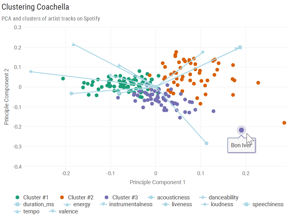

Click to view plot in new window

To see what that third principle component would add (but really just because I couldn’t NOT take this opportunity to make a 3D plot), I used the threejs package to plot the first three principle components, which accounted for 62% of the variance.

library(threejs)

scatterplot3js(pca$x[, 1:3], color : pal[clust], labels : hplot$name, renderer : 'canvas')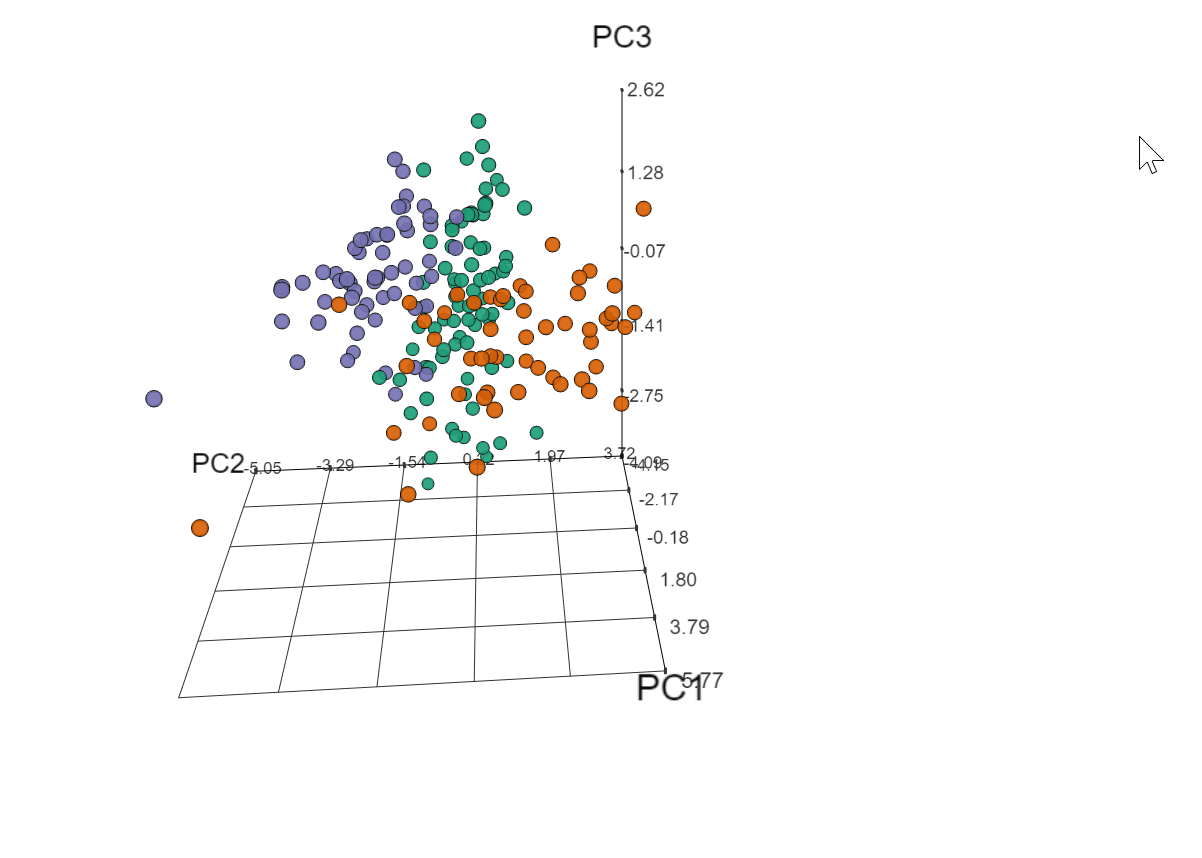

Click to view plot in new window

Yep, totally worth it. Soooo what does it all mean?

Interpreting the Three Clusters

I did a quick exploratory analysis to find simple combinations of audio features that separated the clusters. One plot that stood out was (instrumentalness + danceability) versus (acousticness - valence). You can find Spotify’s methodology here, but as a quick summary: - Instrumentalness: Probability that the track is instrumental (no lyrics) - Danceability: How easy the track is to dance to (0 not at all, 1 boogie down) - Acousticness: Probability the track is acoustic (not electronic) - Valence: Track positivity (0 is sad/angry, 1 is happy/joyous)

cluster_labels <- c('Hip-hop/Rock', 'EDM/Experimental', 'Alternative/Acoustic')

artist_plot_df <- artist_features %>%
    mutate(cluster : paste0('Cluster #', clust, ' - ', cluster_labels[clust]),
           tooltip : artist_name,
           xvar : rescale(instrumentalness + danceability, to : c(0, 1)),
           yvar : rescale(acousticness - energy, to : c(0, 1)))


hchart(artist_plot_df, hcaes(x : xvar, y : yvar, group : cluster), type : 'scatter') %>%
    hc_tooltip(formatter : JS(paste0("function() {return this.point.tooltip;}")), useHTML : T) %>%
    hc_colors(color : pal) %>%
    hc_xAxis(max : 1, title : list(text : 'Instrumentalness + Danceability')) %>%
    hc_yAxis(max : 1, title : list(text : 'Acousticness - Valence')) %>%
    hc_add_theme(hc_theme_smpl()) %>%
    hc_yAxis(plotLines : list(list(
        value : .5,
        color : 'black',
        width : 2,
        zIndex : 2))) %>%
    hc_xAxis(plotLines : list(list(
        value : .5,
        color : 'black',
        width : 2,
        zIndex : 2))) %>%
    hc_title(text : 'The Three Types of Artists at Coachella 2017') %>%
    hc_subtitle(text : HTML('<em>Clustering of their top tracks on Spotify</em>')) %>%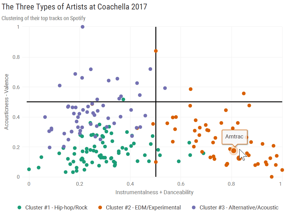

Click to view plot in new window